Exercise XI: Embeddings

Learned Representations & The Geometry of Meaning

Introduction

An embedding is a dense representation where we specifically enforce a geometrical property: similar objects must be closer together in the latent space. This is different from standard dimensionality reduction; here, the “meaning” is learned through specific loss functions, such as contrastive learning.

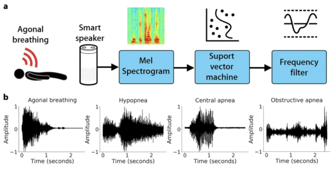
A primary example of this is VGGish, which converts audio spectrograms into feature embeddings that a classifier can use to distinguish between complex signals, such as different types of breathing patterns.

Key Concepts

Semantic Embedding: Learning a dense representation where similar words have similar encodings.

Encoders: Models like DistilBERT (text), VGGish (audio), or CLIP (image/text) act as the “engine” that creates these vectors.

Contrastive Alignment: Models like CLIP align different modalities (images and text) into the same embedding space.

Working with Text Embeddings (DistilBERT)

introduction to DistilBERT

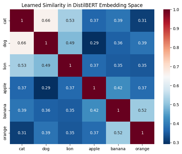
DistilBERT is a pre-trained transformer model that maps text into a 768-dimensional latent space. Each sentence is tokenized and passed through the model to produce a vector that captures its semantic essence.

We can verify the “enforced geometry” of the embedding space by calculating the Cosine Similarity between different concepts.

from sentence_transformers import SentenceTransformer
from sklearn.metrics.pairwise import cosine_similarity
import seaborn as sns
import matplotlib.pyplot as plt

# Load a pre-trained DistilBERT-based model
# This model has already 'learned' the semantic structure of language
model = SentenceTransformer('all-MiniLM-L6-v2') 

# Define stimuli categories
stimuli = ["cat", "dog", "lion", "apple", "banana", "orange"]

# 1. Generate Embeddings (Model Input -> Encoding -> Dense Vector)
embeddings = model.encode(stimuli)

# 2. Compute Similarity Matrix 
# This reveals how the model clusters 'Animals' vs 'Fruits'
sim_matrix = cosine_similarity(embeddings)

# 3. Visualize the geometry
plt.figure(figsize=(8, 6))
sns.heatmap(sim_matrix, xticklabels=stimuli, yticklabels=stimuli, annot=True, cmap='RdBu_r')
plt.title("Learned Similarity in DistilBERT Embedding Space")
plt.show()

Supervised Decoding - Predicting from Embeddings

Introduction

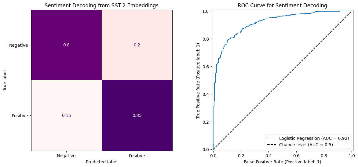
Once we have these learned features, we can use them as inputs for supervised models (e.g., Logistic Regression). In this section, we predict the sentiment of a sentence based solely on its position in the embedding space.

Task: Sentiment Analysis on the SST-2 Dataset

We will use samples from an open-source sentiment dataset to train a classifier.

from sklearn.linear_model import LogisticRegression
from sklearn.model_selection import train_test_split
import pandas as pd

splits = {'train': 'data/train-00000-of-00001.parquet', 'validation': 'data/validation-00000-of-00001.parquet', 'test': 'data/test-00000-of-00001.parquet'}
df = pd.read_parquet("hf://datasets/stanfordnlp/sst2/" + splits["train"])

# sample 3000 rows for demo purposes
df = df.sample(n=3000, random_state=42).reset_index(drop=True)

# 1. Prepare a small labeled dataset for sentiment analysis
sentences = df['sentence'].tolist()
y = df['label'].tolist()  # 0 = negative, 1 = positive

# demonstrate "positive" and "negative" examples
rand_pos = df[df['label'] == 1]['sentence'].sample(3).values
rand_neg = df[df['label'] == 0]['sentence'].sample(3).values

print("Positive Examples:")
for sent in rand_pos:
    print(f" - {sent}")
print("\nNegative Examples:")
for sent in rand_neg:
    print(f" - {sent}")

Positive Examples:
 - a remarkable and novel 
 - have been kind enough to share it 
 - real narrative logic 

Negative Examples:
 - supermarket tabloids 
 - lee 's character did n't just go to a bank manager and save everyone the misery 
 - a choppy ending 

# 2. Generate Embeddings (768 dimensions per sentence)
print("Generating embeddings for 3000 SST-2 samples...")
transformer = SentenceTransformer('all-MiniLM-L6-v2') 
X_embeddings = transformer.encode(sentences)

print(f"Feature Matrix Shape: {X_embeddings.shape} (Samples, Embedding Dim)")

Generating embeddings for 3000 SST-2 samples...

Feature Matrix Shape: (3000, 384) (Samples, Embedding Dim)

# 3. Split into Training and Testing sets (75% / 25%)
from sklearn.metrics import ConfusionMatrixDisplay
from sklearn.metrics import RocCurveDisplay

X_train, X_test, y_train, y_test = train_test_split(
    X_embeddings, y, test_size=0.25, stratify=y, random_state=42
)

# 4. Train a Logistic Regression Classifier
clf = LogisticRegression(max_iter=1000)
clf.fit(X_train, y_train)

# 5. Evaluate the results
y_pred = clf.predict(X_test)

# 6. Visualize the Confusion Matrix and ROC Curve
fig, axes = plt.subplots(1, 2, figsize=(14, 6))
ConfusionMatrixDisplay.from_estimator(clf, X_test, y_test, 
                                      display_labels=['Negative', 'Positive'], 
                                      cmap='RdPu',
                                      normalize='true',
                                      ax=axes[0],
                                      colorbar=False
                                      )
axes[0].set_title("Sentiment Decoding from SST-2 Embeddings")
axes[0].grid(False)

RocCurveDisplay.from_estimator(clf, X_test, y_test, ax=axes[1], name='Logistic Regression', plot_chance_level=True)
axes[1].set_title("ROC Curve for Sentiment Decoding")

Text(0.5, 1.0, 'ROC Curve for Sentiment Decoding')

From Mathematical Embeddings to Neural Representations (RSA)

Embeddings as a Simulation of Semantic Similarity

In this course, we treat embeddings as a mathematical approach trying to simulate the “similarity” in the way the brain processes objects of similar context or semantics. While raw brain activity (e.g., fMRI or ECoG) is a biological response, machine learning models use specific loss functions to enforce a geometrical structure where meaningful relationships are preserved in the distance between vectors.

Representational Similarity Analysis (RSA):

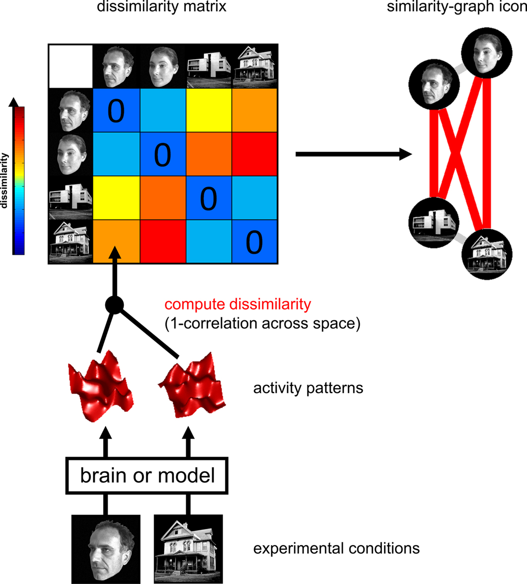
To test if these mathematical simulations match the brain, we use Representational Similarity Analysis (RSA)\(^1\).

Model Similarity: We create a similarity matrix (like in Part 2) showing how the model represents a set of stimuli.

Brain Similarity: We create a second similarity matrix based on neural responses to those same stimuli.

Comparison: We correlate these two matrices. A high correlation suggests that the machine embedding captures a “brain-like” representation of the information.

⚠️ A Final Distinction

Neural Activity: This is the raw biological signal. We do not automatically call it an “embedding” unless we have demonstrated that it satisfies learned geometrical properties.

Machine Embeddings: These are engineered features. We use them as a proxy or a hypothesis of how the brain might be organizing information.

[1] Kriegeskorte, N., Mur, M., & Bandettini, P. A. (2008). Representational similarity analysis-connecting the branches of systems neuroscience. Frontiers in systems neuroscience, 2, 249.