Exercise II: k-Nearest Neighbors (k-NN)#
k-NN is a simple and useful non-parametric method that is commonly used for both classification and regression. It relies on having some method of calculating distance between data points, and using the the “nearest” observations to predict the target value for new ones.

The Curse of Dimensionality
The curse of dimensionality refers to various phenomena that arise when analyzing and organizing data in high-dimensional spaces that do not occur in low-dimensional settings such as the three-dimensional physical space of everyday experience. Wikipedia
k-NN normally performs better with a limited number of features. In simplified terms, distances become increasingly large in higher dimensionality spaces.
Loading the Dataset#
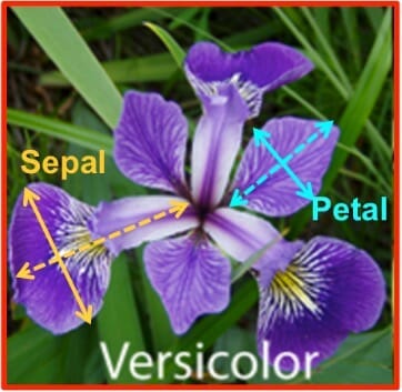
In this exercise we will use the Iris Flower Dataset. This dataset is commonly used for demonstrating simple statistical concepts and therefore scikit-learn provides us with a utility function to load it.
import pandas as pd

from sklearn.datasets import load_iris

TARGET_NAME = "class"

# Read a type of dictionary with the dataset as well as some metadata.
iris_dataset = load_iris()

# Read the features and targets.
X = pd.DataFrame(iris_dataset.data, columns=iris_dataset.feature_names)
y = pd.Series(iris_dataset.target, name=TARGET_NAME)
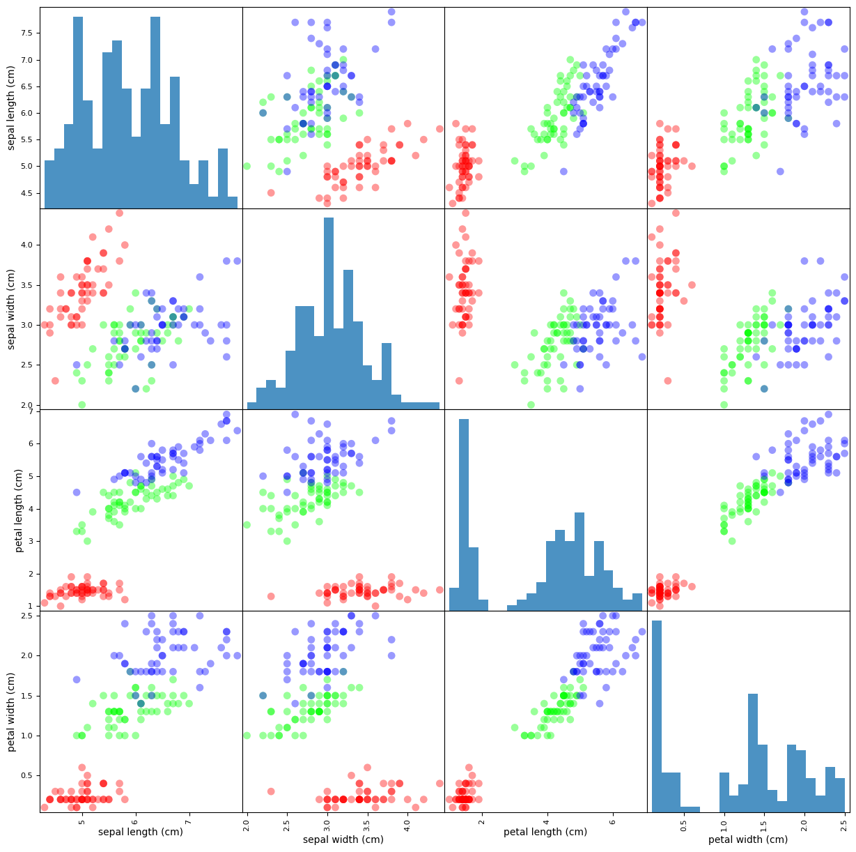
Basic Exploration#
print(iris_dataset.DESCR)
.. _iris_dataset:

Iris plants dataset
--------------------

**Data Set Characteristics:**

:Number of Instances: 150 (50 in each of three classes)
:Number of Attributes: 4 numeric, predictive attributes and the class
:Attribute Information:
    - sepal length in cm
    - sepal width in cm
    - petal length in cm
    - petal width in cm
    - class:
            - Iris-Setosa
            - Iris-Versicolour
            - Iris-Virginica

:Summary Statistics:

============== ==== ==== ======= ===== ====================
                Min  Max   Mean    SD   Class Correlation
============== ==== ==== ======= ===== ====================
sepal length:   4.3  7.9   5.84   0.83    0.7826
sepal width:    2.0  4.4   3.05   0.43   -0.4194
petal length:   1.0  6.9   3.76   1.76    0.9490  (high!)
petal width:    0.1  2.5   1.20   0.76    0.9565  (high!)
============== ==== ==== ======= ===== ====================

:Missing Attribute Values: None
:Class Distribution: 33.3% for each of 3 classes.
:Creator: R.A. Fisher
:Donor: Michael Marshall (MARSHALL%PLU@io.arc.nasa.gov)
:Date: July, 1988

The famous Iris database, first used by Sir R.A. Fisher. The dataset is taken
from Fisher's paper. Note that it's the same as in R, but not as in the UCI
Machine Learning Repository, which has two wrong data points.

This is perhaps the best known database to be found in the
pattern recognition literature.  Fisher's paper is a classic in the field and
is referenced frequently to this day.  (See Duda & Hart, for example.)  The
data set contains 3 classes of 50 instances each, where each class refers to a
type of iris plant.  One class is linearly separable from the other 2; the
latter are NOT linearly separable from each other.

.. dropdown:: References

  - Fisher, R.A. "The use of multiple measurements in taxonomic problems"
    Annual Eugenics, 7, Part II, 179-188 (1936); also in "Contributions to
    Mathematical Statistics" (John Wiley, NY, 1950).
  - Duda, R.O., & Hart, P.E. (1973) Pattern Classification and Scene Analysis.
    (Q327.D83) John Wiley & Sons.  ISBN 0-471-22361-1.  See page 218.
  - Dasarathy, B.V. (1980) "Nosing Around the Neighborhood: A New System
    Structure and Classification Rule for Recognition in Partially Exposed
    Environments".  IEEE Transactions on Pattern Analysis and Machine
    Intelligence, Vol. PAMI-2, No. 1, 67-71.
  - Gates, G.W. (1972) "The Reduced Nearest Neighbor Rule".  IEEE Transactions
    on Information Theory, May 1972, 431-433.
  - See also: 1988 MLC Proceedings, 54-64.  Cheeseman et al"s AUTOCLASS II
    conceptual clustering system finds 3 classes in the data.
  - Many, many more ...
| sepal length (cm) | sepal width (cm) | petal length (cm) | petal width (cm) | class | |
|---|---|---|---|---|---|
| 0 | 5.10 | 3.50 | 1.40 | 0.20 | setosa |
| 1 | 4.90 | 3.00 | 1.40 | 0.20 | setosa |
| 2 | 4.70 | 3.20 | 1.30 | 0.20 | setosa |
| 3 | 4.60 | 3.10 | 1.50 | 0.20 | setosa |
| 4 | 5.00 | 3.60 | 1.40 | 0.20 | setosa |
| 72 | 6.30 | 2.50 | 4.90 | 1.50 | versicolor |
| 73 | 6.10 | 2.80 | 4.70 | 1.20 | versicolor |
| 74 | 6.40 | 2.90 | 4.30 | 1.30 | versicolor |
| 75 | 6.60 | 3.00 | 4.40 | 1.40 | versicolor |
| 76 | 6.80 | 2.80 | 4.80 | 1.40 | versicolor |
| 145 | 6.70 | 3.00 | 5.20 | 2.30 | virginica |
| 146 | 6.30 | 2.50 | 5.00 | 1.90 | virginica |
| 147 | 6.50 | 3.00 | 5.20 | 2.00 | virginica |
| 148 | 6.20 | 3.40 | 5.40 | 2.30 | virginica |
| 149 | 5.90 | 3.00 | 5.10 | 1.80 | virginica |
X.info()
<class 'pandas.core.frame.DataFrame'>
RangeIndex: 150 entries, 0 to 149
Data columns (total 4 columns):
 #   Column             Non-Null Count  Dtype
---  ------             --------------  -----
 0   sepal length (cm)  150 non-null    float64
 1   sepal width (cm)   150 non-null    float64
 2   petal length (cm)  150 non-null    float64
 3   petal width (cm)   150 non-null    float64
dtypes: float64(4)
memory usage: 4.8 KB
X.describe()
| sepal length (cm) | sepal width (cm) | petal length (cm) | petal width (cm) | |
|---|---|---|---|---|
| count | 150.000000 | 150.000000 | 150.000000 | 150.000000 |
| mean | 5.843333 | 3.057333 | 3.758000 | 1.199333 |
| std | 0.828066 | 0.435866 | 1.765298 | 0.762238 |
| min | 4.300000 | 2.000000 | 1.000000 | 0.100000 |
| 25% | 5.100000 | 2.800000 | 1.600000 | 0.300000 |
| 50% | 5.800000 | 3.000000 | 4.350000 | 1.300000 |
| 75% | 6.400000 | 3.300000 | 5.100000 | 1.800000 |
| max | 7.900000 | 4.400000 | 6.900000 | 2.500000 |
Train/Test Split#
A lot can be said regarding the different approaches for model validation and evaluation (which we’ll discuss later in the course), but the general guideline is that, since our model should detect underlying trends in the data, we would evaluate its performance over unseen data. Therefore, we’ll split our data into a training (for model fitting) and testing (for evaluation).
from sklearn.model_selection import train_test_split

X_train, X_test, y_train, y_test = train_test_split(X,
                                                    y,
                                                    random_state=0,
                                                    test_size=0.25)
We now have a training dataset consisting of 112 observations and a test dataset with 38 observations.
Model Creation#
Machine Learning algorithms and models are easily accesible through numberous packages, namely scikit-learn. While different estimators provide different advantages and pitfalls, they share some basic properties, making it easy for users to use them.
*Since these estimators are basically just algorithms and formulas that need to be tailored to the dataset being used, all estimators have a ‘fit’ method, (unsurprisingly) fitting the estimators to generalize to any specific data.
from sklearn.neighbors import KNeighborsClassifier

k = 1

knn = KNeighborsClassifier(n_neighbors=k)
_ = knn.fit(X_train, y_train)
Model Evaluation#
Misclassification Rate / Accuracy#

import numpy as np

y_predicted = knn.predict(X_test)

misclassification_rate = np.mean(y_predicted != y_test) * 100
Our model achieved a misclassification_rate of ‘2.632’%, meaning it correctly predicted np.int64(37) of 38 target values in our test set.
Another way to look at it is:
from sklearn.metrics import accuracy_score
accuracy_score(y_test, y_predicted) * 100
97.36842105263158
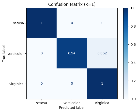
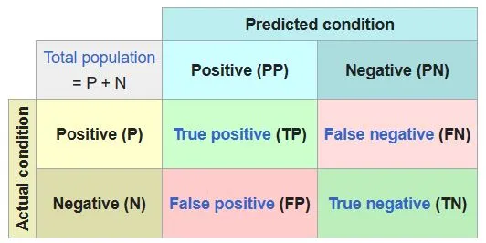
Confusion Matrix#
from sklearn.metrics import confusion_matrix
confusion_matrix(y_test, y_predicted)
array([[13,  0,  0],
       [ 0, 15,  1],
       [ 0,  0,  9]])
import matplotlib.pyplot as plt

from sklearn.metrics import ConfusionMatrixDisplay


disp = ConfusionMatrixDisplay.from_estimator(knn,
                             X_test,
                             y_test,
                             display_labels=iris_dataset.target_names,
                             cmap=plt.cm.Blues,
                             normalize="true")
_ = disp.ax_.set_title(f"Confusion Matrix (k={k})")