Exercise VII: Decision Trees and Random Forests#
Decision trees are as easy to implement with sklearn as any other of the models we’ve studied so far. As a quick example we could try to classify the iris dataset which we’re already familiar with:
decision_tree = DecisionTreeClassifier(random_state=42)
_ = decision_tree.fit(X_train, y_train)
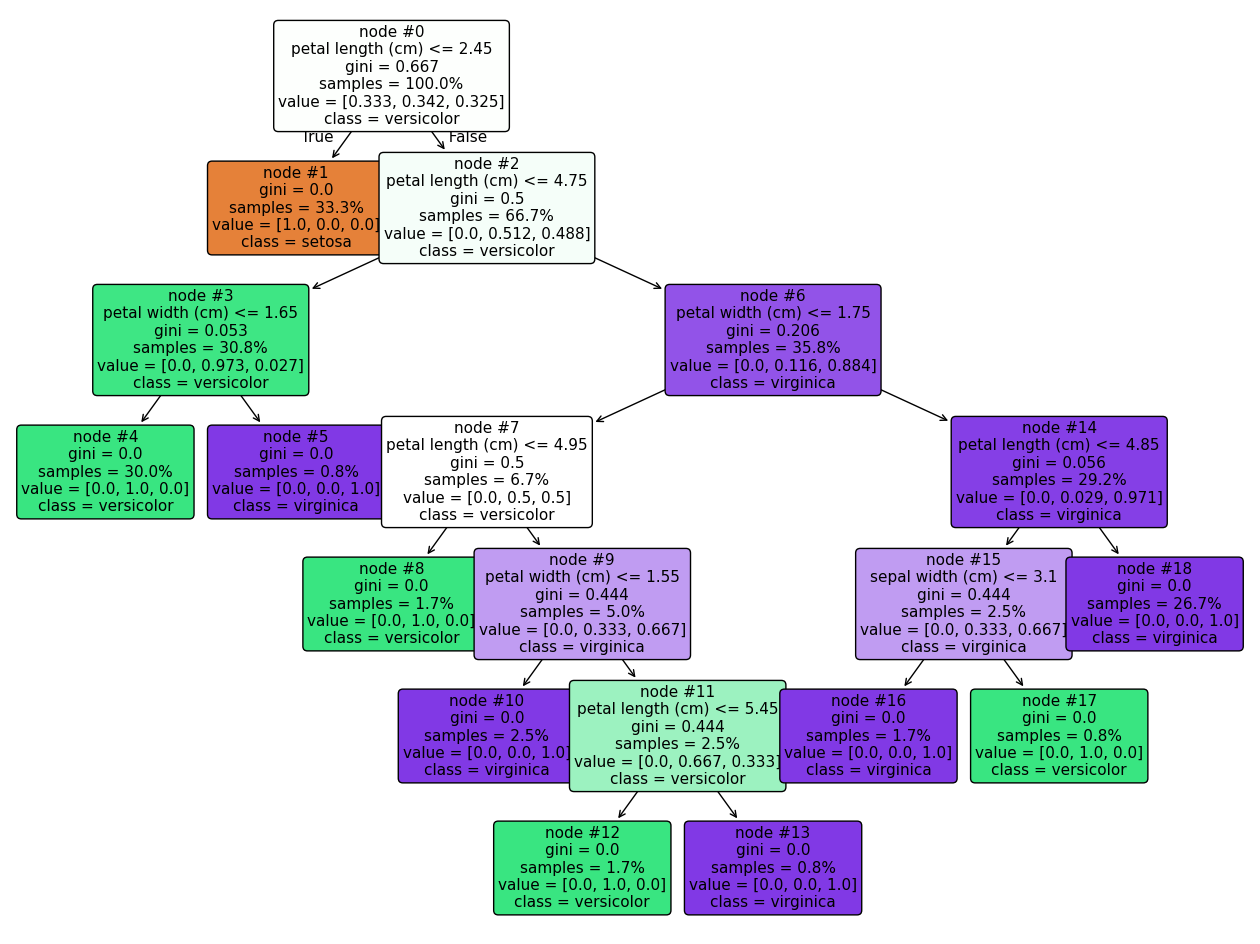
Trees are even easy to visualize, thanks to the plot_tree() function:
import matplotlib.pyplot as plt

fig, ax = plt.subplots(figsize=(16, 12))
_ = plot_tree(decision_tree,
              class_names=data["target_names"].tolist(),
              feature_names=data["feature_names"],
              filled=True,
              fontsize=11,
              node_ids=True,
              proportion=True,
              rounded=True,
              ax=ax)
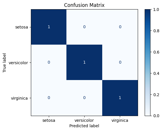
Finally, we can evaluate the model’s performance using the appropriate metrics, e.g.:
from sklearn.metrics import ConfusionMatrixDisplay

disp = ConfusionMatrixDisplay.from_estimator(decision_tree,
                                             X_test,
                                             y_test,
                                             cmap=plt.cm.Blues,
                                             normalize="true",
                                             display_labels=data["target_names"])
disp.ax_.set_title("Confusion Matrix")
Text(0.5, 1.0, 'Confusion Matrix')
from sklearn.metrics import classification_report

y_predicted = decision_tree.predict(X_test)
print(classification_report(y_test, y_predicted))
              precision    recall  f1-score   support

      setosa       1.00      1.00      1.00        10
  versicolor       1.00      1.00      1.00         9
   virginica       1.00      1.00      1.00        11

    accuracy                           1.00        30
   macro avg       1.00      1.00      1.00        30
weighted avg       1.00      1.00      1.00        30
Predicting ASD Diagnosis:#
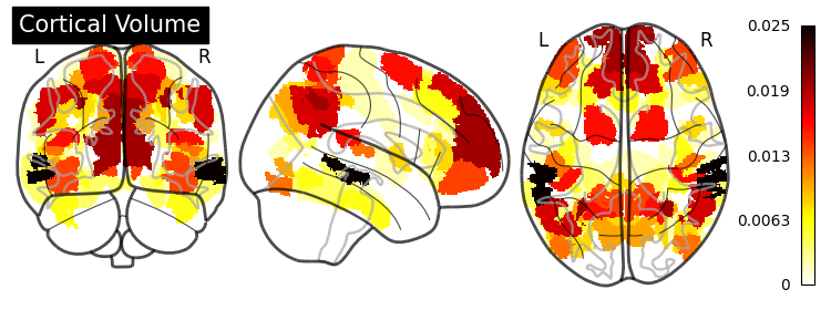
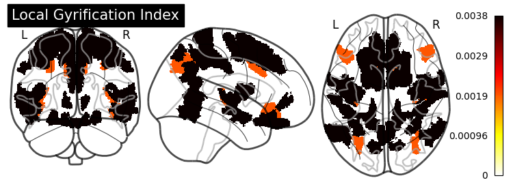
Again, we will try and create a model to classify ASD diagnosis using four FreeSurfer metrics extracted over 360 brain regions. In the previous exercise we used an \(\ell_2\) regularized logistic regression model (estimated using the LogisticRegressionCV class) to select and fit a model, this time we will use the RandomForestClassifier and GradientBoostingClassifier to do the same.
Random Forest#
Model Creation#
from sklearn.ensemble import RandomForestClassifier

random_forest = RandomForestClassifier(random_state=0)
_ = random_forest.fit(X_train, y_train)
Model Application#
y_predicted = random_forest.predict(X_test)
Model Evaluation#
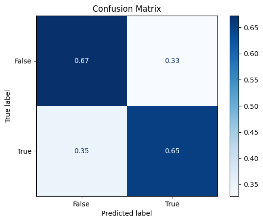
Confusion Matrix#
disp = ConfusionMatrixDisplay.from_estimator(random_forest,
                                             X_test,
                                             y_test,
                                             cmap=plt.cm.Blues,
                                             normalize="true")
disp.ax_.set_title("Confusion Matrix")
Text(0.5, 1.0, 'Confusion Matrix')
Classification Report#
print(classification_report(y_test, y_predicted))
              precision    recall  f1-score   support

       False       0.68      0.72      0.70        58
        True       0.62      0.57      0.59        46

    accuracy                           0.65       104
   macro avg       0.65      0.64      0.65       104
weighted avg       0.65      0.65      0.65       104
Not too bad! We’ve improved our accuracy from 0.63 to 0.65.
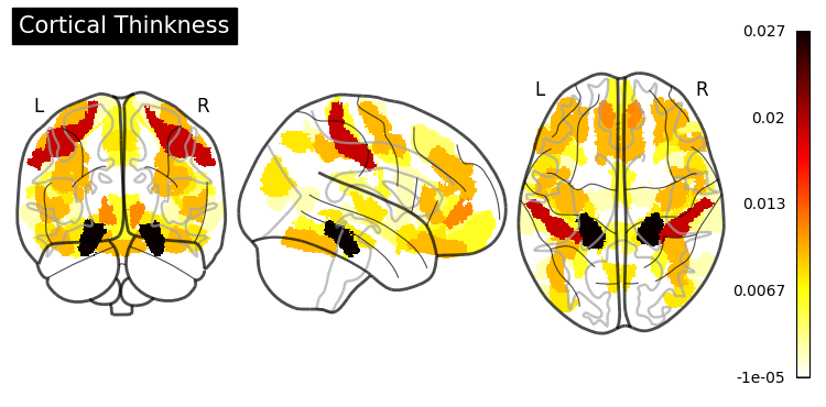
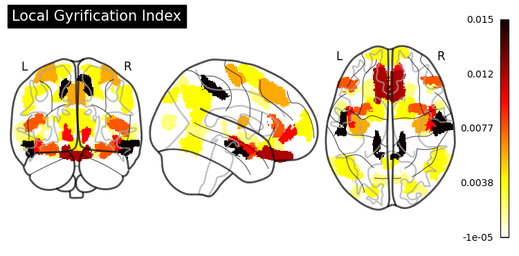
Feature Importance#
One of the greatest things about trees is their interpretability. sklearn exposes one measure (“Gini importance”) as a built-in property of the fitted random forest estimator:
random_forest.feature_importances_
array([2.96342846e-04, 5.08910846e-05, 6.69469236e-04, ...,
       5.30759983e-04, 2.16033616e-04, 4.88856474e-04], shape=(1440,))
However, the documentation states that:
“impurity-based feature importances can be misleading for high cardinality features (many unique values).”
In our case, having numerical features, we would be better off using the permutation_importance() function (for more information, see Permutation Importance vs Random Forest Feature Importance).
from sklearn.inspection import permutation_importance

importance = permutation_importance(random_forest,
                                    X_test,
                                    y_test,
                                    random_state=0,
                                    n_jobs=8)
---------------------------------------------------------------------------
KeyboardInterrupt                         Traceback (most recent call last)
Cell In[12], line 3
      1 from sklearn.inspection import permutation_importance
----> 3 importance = permutation_importance(random_forest,
      4                                     X_test,
      5                                     y_test,
      6                                     random_state=0,
      7                                     n_jobs=8)

File /opt/hostedtoolcache/Python/3.11.14/x64/lib/python3.11/site-packages/sklearn/utils/_param_validation.py:218, in validate_params.<locals>.decorator.<locals>.wrapper(*args, **kwargs)
    212 try:
    213     with config_context(
    214         skip_parameter_validation=(
    215             prefer_skip_nested_validation or global_skip_validation
    216         )
    217     ):
--> 218         return func(*args, **kwargs)
    219 except InvalidParameterError as e:
    220     # When the function is just a wrapper around an estimator, we allow
    221     # the function to delegate validation to the estimator, but we replace
    222     # the name of the estimator by the name of the function in the error
    223     # message to avoid confusion.
    224     msg = re.sub(
    225         r"parameter of \w+ must be",
    226         f"parameter of {func.__qualname__} must be",
    227         str(e),
    228     )

File /opt/hostedtoolcache/Python/3.11.14/x64/lib/python3.11/site-packages/sklearn/inspection/_permutation_importance.py:288, in permutation_importance(estimator, X, y, scoring, n_repeats, n_jobs, random_state, sample_weight, max_samples)
    285 scorer = check_scoring(estimator, scoring=scoring)
    286 baseline_score = _weights_scorer(scorer, estimator, X, y, sample_weight)
--> 288 scores = Parallel(n_jobs=n_jobs)(
    289     delayed(_calculate_permutation_scores)(
    290         estimator,
    291         X,
    292         y,
    293         sample_weight,
    294         col_idx,
    295         random_seed,
    296         n_repeats,
    297         scorer,
    298         max_samples,
    299     )
    300     for col_idx in range(X.shape[1])
    301 )
    303 if isinstance(baseline_score, dict):
    304     return {
    305         name: _create_importances_bunch(
    306             baseline_score[name],
   (...)    310         for name in baseline_score
    311     }

File /opt/hostedtoolcache/Python/3.11.14/x64/lib/python3.11/site-packages/sklearn/utils/parallel.py:91, in Parallel.__call__(self, iterable)
     79 warning_filters = (
     80     filters_func() if filters_func is not None else warnings.filters
     81 )
     83 iterable_with_config_and_warning_filters = (
     84     (
     85         _with_config_and_warning_filters(delayed_func, config, warning_filters),
   (...)     89     for delayed_func, args, kwargs in iterable
     90 )
---> 91 return super().__call__(iterable_with_config_and_warning_filters)

File /opt/hostedtoolcache/Python/3.11.14/x64/lib/python3.11/site-packages/joblib/parallel.py:2072, in Parallel.__call__(self, iterable)
   2066 # The first item from the output is blank, but it makes the interpreter
   2067 # progress until it enters the Try/Except block of the generator and
   2068 # reaches the first `yield` statement. This starts the asynchronous
   2069 # dispatch of the tasks to the workers.
   2070 next(output)
-> 2072 return output if self.return_generator else list(output)

File /opt/hostedtoolcache/Python/3.11.14/x64/lib/python3.11/site-packages/joblib/parallel.py:1682, in Parallel._get_outputs(self, iterator, pre_dispatch)
   1679     yield
   1681     with self._backend.retrieval_context():
-> 1682         yield from self._retrieve()
   1684 except GeneratorExit:
   1685     # The generator has been garbage collected before being fully
   1686     # consumed. This aborts the remaining tasks if possible and warn
   1687     # the user if necessary.
   1688     self._exception = True

File /opt/hostedtoolcache/Python/3.11.14/x64/lib/python3.11/site-packages/joblib/parallel.py:1800, in Parallel._retrieve(self)
   1789 if self.return_ordered:
   1790     # Case ordered: wait for completion (or error) of the next job
   1791     # that have been dispatched and not retrieved yet. If no job
   (...)   1795     # control only have to be done on the amount of time the next
   1796     # dispatched job is pending.
   1797     if (nb_jobs == 0) or (
   1798         self._jobs[0].get_status(timeout=self.timeout) == TASK_PENDING
   1799     ):
-> 1800         time.sleep(0.01)
   1801         continue
   1803 elif nb_jobs == 0:
   1804     # Case unordered: jobs are added to the list of jobs to
   1805     # retrieve `self._jobs` only once completed or in error, which
   (...)   1811     # timeouts before any other dispatched job has completed and
   1812     # been added to `self._jobs` to be retrieved.

KeyboardInterrupt:

Gradient Boosting#
Model Creation#
from sklearn.ensemble import GradientBoostingClassifier

gradient_boosting = GradientBoostingClassifier(random_state=0)
_ = gradient_boosting.fit(X_train, y_train)
Model Application#
y_predicted_gb = gradient_boosting.predict(X_test)
Model Evaluation#
Confusion Matrix#
disp = ConfusionMatrixDisplay.from_estimator(gradient_boosting,
                                             X_test,
                                             y_test,
                                             cmap=plt.cm.Blues,
                                             normalize="true")
disp.ax_.set_title("Confusion Matrix")
Text(0.5, 1.0, 'Confusion Matrix')
Classification Report#
print(classification_report(y_test, y_predicted_gb))
              precision    recall  f1-score   support

       False       0.71      0.67      0.69        58
        True       0.61      0.65      0.63        46

    accuracy                           0.66       104
   macro avg       0.66      0.66      0.66       104
weighted avg       0.67      0.66      0.66       104
We’ve ended up with an overall slightly better accuracy and precision.
Feature Importance#
from sklearn.inspection import permutation_importance

gb_importance = permutation_importance(gradient_boosting,
                                       X_test,
                                       y_test,
                                       random_state=0,
                                       n_jobs=8)


Hyperparameter Tuning#
Grid Search#
from sklearn.model_selection import GridSearchCV

N_ESTIMATORS = range(60, 130, 10)
MAX_DEPTH = range(2, 5)
PARAM_GRID = {"n_estimators": N_ESTIMATORS, "max_depth": MAX_DEPTH}

estimator = GradientBoostingClassifier(random_state=0)
model_searcher = GridSearchCV(estimator,
                              param_grid=PARAM_GRID,
                              return_train_score=True)
Model Selection#
_ = model_searcher.fit(X_train, y_train)
Selected Model Application#
y_predicted_grid = model_searcher.predict(X_test)
Selected Model Evaluation#
model_searcher.best_params_
{'max_depth': 3, 'n_estimators': 70}
model_searcher.best_score_
0.6355555555555555
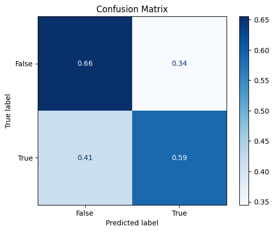
Confusion Matrix#
disp = ConfusionMatrixDisplay.from_estimator(model_searcher,
                                             X_test,
                                             y_test,
                                             cmap=plt.cm.Blues,
                                             normalize="true")
disp.ax_.set_title("Confusion Matrix")
Text(0.5, 1.0, 'Confusion Matrix')
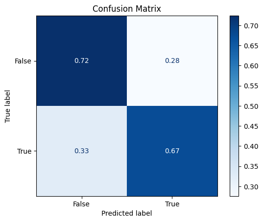
Classification Report#
print(classification_report(y_test, y_predicted_grid))
              precision    recall  f1-score   support

       False       0.74      0.72      0.73        58
        True       0.66      0.67      0.67        46

    accuracy                           0.70       104
   macro avg       0.70      0.70      0.70       104
weighted avg       0.70      0.70      0.70       104
Model Selection#
COLORS = "red", "green", "blue"
PARAM_COLUMNS = [
    "param_max_depth", "param_n_estimators", "mean_train_score",
    "mean_test_score", "std_train_score", "std_test_score"
]
PARAM_COLUMN_NAMES = [
    "Max Depth", "Number of Estimators", "Mean Train Score", "Mean Test Score",
    "Train Score STD", "Test Score STD"
]


def plot_search_results(cv_results: dict):
    data = pd.DataFrame(cv_results)[PARAM_COLUMNS].copy()
    data.columns = PARAM_COLUMN_NAMES
    param_fig, param_ax = plt.subplots(figsize=(10, 5))
    param_ax.set_title(
        "GridSearchCV Test-set Accuracy by Number of Estimators and Max. Depth"
    )

    for i, (key, grp) in enumerate(data.groupby(["Max Depth"])):
        grp.plot(kind="line",
                 x="Number of Estimators",
                 y="Mean Test Score",
                 color=COLORS[i],
                 label=str(key),
                 ax=param_ax)
        score_mean = grp["Mean Test Score"]
        score_std = grp["Test Score STD"]
        score_lower_limit = score_mean - score_std
        score_upper_limit = score_mean + score_std
        param_ax.fill_between(grp["Number of Estimators"],
                              score_lower_limit,
                              score_upper_limit,
                              color=COLORS[i],
                              alpha=0.1)
    param_ax.set_ylabel("Accuracy")
    param_ax.scatter(model_searcher.best_params_["n_estimators"],
                     model_searcher.best_score_,
                     marker="*",
                     color="black",
                     s=150,
                     label="Selected Model")
    _ = param_ax.legend()
plot_search_results(model_searcher.cv_results_)
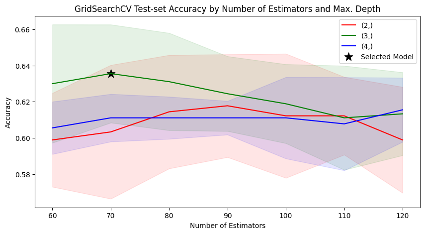
What would happen if we changed cv from it’s default value (5) to 10? Would GridSearchCV select the same model?
model_searcher_2 = GridSearchCV(estimator,
                                param_grid=PARAM_GRID,
                                return_train_score=True,
                                cv=10)
Model Selection#
_ = model_searcher_2.fit(X_train, y_train)
Selected Model Application#
y_predicted_grid_2 = model_searcher_2.predict(X_test)
Selected Model Evaluation#
model_searcher_2.best_params_
{'max_depth': 3, 'n_estimators': 120}
model_searcher_2.best_score_
0.6199999999999999
Confusion Matrix#
disp = ConfusionMatrixDisplay.from_estimator(model_searcher_2,
                                             X_test,
                                             y_test,
                                             cmap=plt.cm.Blues,
                                             normalize="true")
disp.ax_.set_title("Confusion Matrix")
Text(0.5, 1.0, 'Confusion Matrix')
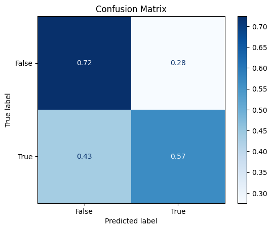
Classification Report#
print(classification_report(y_test, y_predicted_grid_2))
              precision    recall  f1-score   support

       False       0.67      0.66      0.66        58
        True       0.57      0.59      0.58        46

    accuracy                           0.62       104
   macro avg       0.62      0.62      0.62       104
weighted avg       0.63      0.62      0.63       104
Feature Importance#
grid_importance = permutation_importance(model_searcher_2,
                                         X_test,
                                         y_test,
                                         random_state=0,
                                         n_jobs=8)
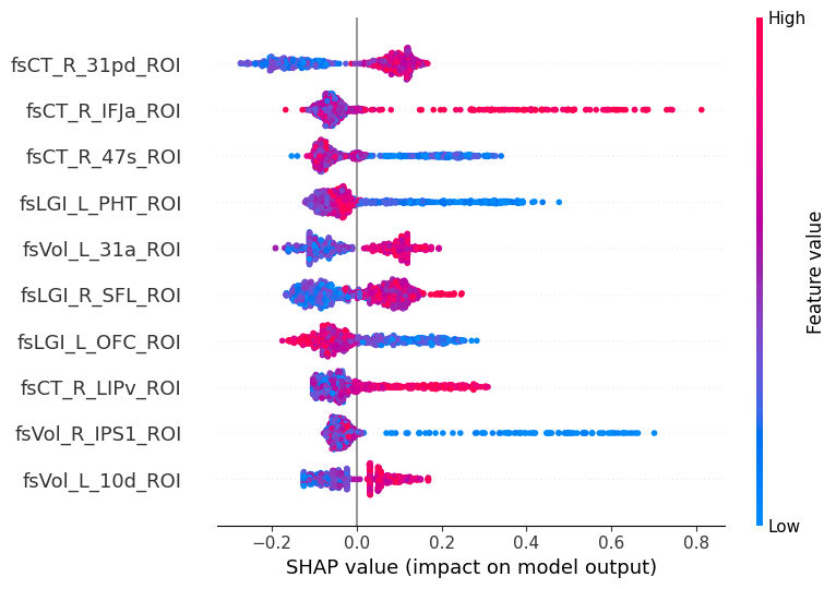
SHAP (SHapley Additive exPlanations) values show how each feature affects each final prediction, the significance of each feature compared to others, and the model’s reliance on the interaction between features:
import shap
shap_values = shap.TreeExplainer(model_searcher_2.best_estimator_).shap_values(X_train)
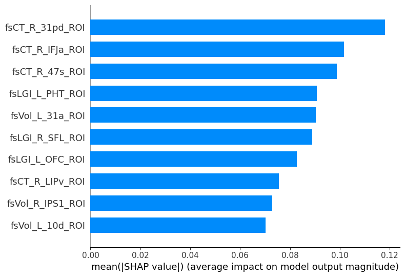
shap.summary_plot(shap_values, X_train, plot_type="bar", max_display=10)
shap.summary_plot(shap_values, X_train, max_display=10)