Exercise IV: Logistic Regression

In statistics, the logistic model (or logit model) is used to model the probability of a certain class or event existing such as pass/fail, win/lose, alive/dead or healthy/sick. This can be extended to model several classes of events such as determining whether an image contains a cat, dog, lion, etc. Each object being detected in the image would be assigned a probability between 0 and 1, with a sum of one. Wikipedia

In this exercise we will reproduce the bank defaults example used in chapter IV of the ISLR, as adapted from the ISLR-python repository.

We will use this example to illustrate the concept of classification, where we aim to predict whether an individual will default on his or her credit card payment (i.e, fail to pay at least the minimal amount in a given number of days).

Setup

Show code cell source

Hide code cell source

import warnings
warnings.simplefilter("ignore")

import pandas as pd

URL = "https://github.com/JWarmenhoven/ISLR-python/raw/master/Notebooks/Data/Default.xlsx"
df = pd.read_excel(URL, index_col=0, true_values=["Yes"], false_values=["No"])

def color_booleans(value: bool) -> str:
    color = "green" if value else "red"
    return f"color: {color}"

BOOLEAN_COLUMNS = ["default", "student"]

df.sample(15).style.text_gradient(cmap="Blues").applymap(color_booleans, subset=BOOLEAN_COLUMNS)

	default	student	balance	income
4117	False	True	1302.340309	16292.267141
3707	False	False	913.638327	50351.155195
9708	False	False	452.367912	29254.871016
7307	False	False	895.746675	35531.837087
9032	False	False	333.180057	29400.477847
5848	False	True	571.577122	15325.079101
4433	False	False	825.287866	46147.955753
8933	False	False	167.584157	49087.255695
118	False	False	1114.403237	47714.022108
5639	False	True	740.228677	23469.387504
6904	False	False	1010.421141	46217.809556
1644	False	True	1255.748135	12209.577068
2246	False	False	1477.669207	42011.807962
7886	False	False	865.886544	59740.732530
194	False	True	1802.903334	21411.423949

There seem to be some imbalance in the number of “default” observations - it seems like most of the individuals in this dataset do not default on their credit card payment.

We will address this issue later on.

display(df["default"].value_counts(normalize=True).to_frame().style.format("{:.2%}").set_caption("Default Rate"))

Default Rate

	proportion
default
False	96.67%
True	3.33%

Feature Scaling

import numpy as np
from sklearn.preprocessing import StandardScaler

numeric_features = df.select_dtypes(include="number")
scaler = StandardScaler()
df.loc[:, numeric_features.columns] = scaler.fit_transform(df.loc[:, numeric_features.columns])

Raw inspection

df.info()

<class 'pandas.core.frame.DataFrame'>
Index: 10000 entries, 1 to 10000
Data columns (total 4 columns):
 #   Column   Non-Null Count  Dtype  
---  ------   --------------  -----  
 0   default  10000 non-null  bool   
 1   student  10000 non-null  bool   
 2   balance  10000 non-null  float64
 3   income   10000 non-null  float64
dtypes: bool(2), float64(2)
memory usage: 253.9 KB

pd.set_option('float_format', '{:g}'.format)
df.describe()

	balance	income
count	10000	10000
mean	-1.24345e-16	3.51008e-16
std	1.00005	1.00005
min	-1.72708	-2.45539
25%	-0.731136	-0.913058
50%	-0.0242674	0.0776593
75%	0.684184	0.771653
max	3.76056	3.0022

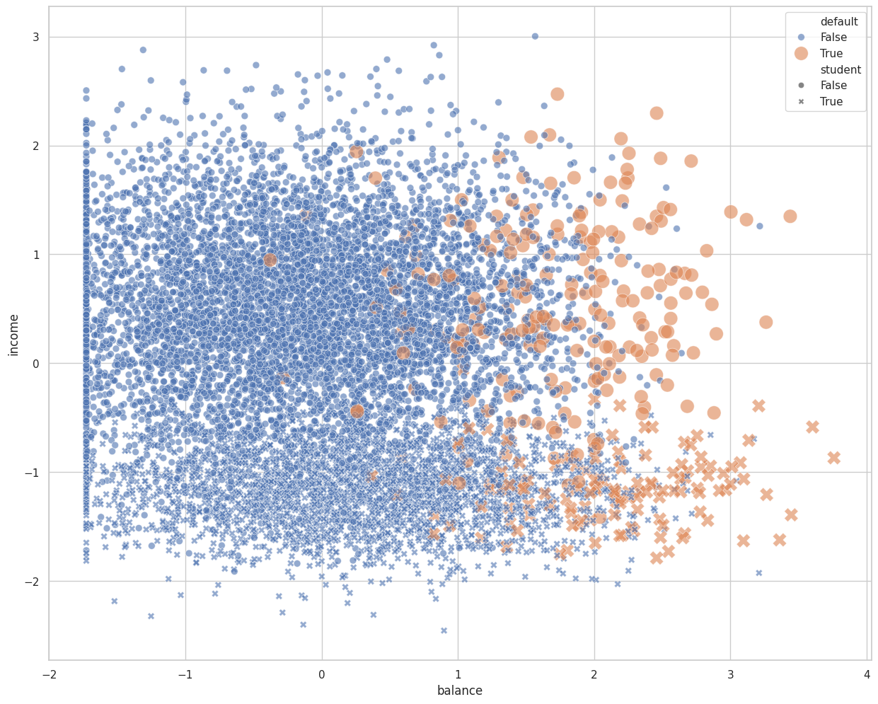
Scatter plot

Visualize some interesting numeric features (balance & income) in relation to our target.

import matplotlib.pyplot as plt
import seaborn as sns
sns.set_theme(style="whitegrid")

fix, ax = plt.subplots(figsize=(15, 12))
_ = sns.scatterplot(x="balance",
                    y="income",
                    hue="default",
                    style="student",
                    size="default",
                    sizes={
                        True: 200,
                        False: 50
                    },
                    alpha=0.6,
                    ax=ax,
                    data=df)

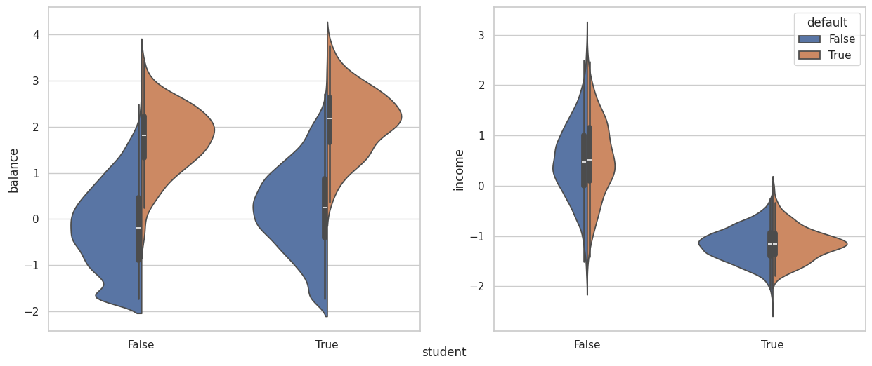
Violin plot

And plot the distributions of these features under each level of the categorical features.

# Create a new figure with two horizontal subplots 
fig, ax = plt.subplots(ncols=2, figsize=(15, 6))

# Plot balance
sns.violinplot(x="student", y="balance", hue="default", split=True, legend=False, ax=ax[0], data=df)
ax[0].set_xlabel('')

# Plot income
sns.violinplot(x="student", y="income", hue="default", split=True, ax=ax[1], data=df)
ax[1].set_xlabel('')

# Add common label
_ = fig.text(0.5, 0.05, "student", ha='center')

Train/Test Split

from sklearn.model_selection import train_test_split 

FEATURE_NAMES = ["balance", "income", "student"]
TARGET_NAME = "default"
X = df[FEATURE_NAMES]
y = df[TARGET_NAME].values

X_train, X_test, y_train, y_test = train_test_split(X,
                                                    y,
                                                    random_state=0,
                                                    test_size=0.2)

Model Creation

sklearn

from sklearn.linear_model import LogisticRegression

sk_model = LogisticRegression(random_state=0, penalty=None, solver="newton-cg")
_ = sk_model.fit(X_train, y_train)

statsmodels

import statsmodels.api as sm

# statsmodels requires booelean values to be converted to integers.
df["student"] = df["student"].astype(int)
df["default"] = df["default"].astype(int)

# R-style model formulation.
sm_model = sm.Logit.from_formula('default ~ balance + income + student', data=df)

Model Application

sklearn

We can predict the probability estimates of each target class (in our case True or False) using the LogisticRegression class’s predict_proba() method:

default_probability = sk_model.predict_proba(X_test)

Note that when predicting probabilities, we get an array of shape \(n_{samples} \text{ X } n_{classes}\), representing the probability of each sample to belong to each class of the target variable.

Or, we could directly return the predictions based on the maximal probabilities:

predictions = sk_model.predict(X_test)

# Manually returning the index of the maximal value
predictions_manual = default_probability.argmax(axis=1)

np.array_equal(predictions, predictions_manual)

True

statsmodels

sm_estimation = sm_model.fit()

Optimization terminated successfully.
         Current function value: 0.078577
         Iterations 10

Model Evaluation

sklearn

print(f"Intercept: {sk_model.intercept_}")
print(f"Coefficients: {sk_model.coef_}")

Intercept: [-5.92939642]
Coefficients: [[ 2.71890021 -0.02275812 -0.61743409]]

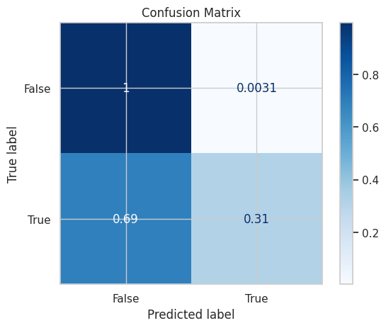
Confusion Matrix

Calculation

from sklearn.metrics import confusion_matrix

confusion_matrix_ = confusion_matrix(y_test, predictions)
print(confusion_matrix_)

[[1920    6]
 [  51   23]]

Visualization

# visualizing the confusion matrix
from sklearn.metrics import ConfusionMatrixDisplay

disp = ConfusionMatrixDisplay.from_estimator(
    sk_model,
    X_test,
    y_test,
    display_labels=sk_model.classes_,
    cmap = plt.cm.Blues,
    normalize="true"
    )
_ = disp.ax_.set_title(f"Confusion Matrix")
# from sklearn.metrics import plot_confusion_matrix

# disp = plot_confusion_matrix(sk_model,
#                              X_test,
#                              y_test,
#                              cmap=plt.cm.Greens,
#                              normalize="true")
# _ = disp.ax_.set_title(f"Confusion Matrix")

Classification Report

from sklearn.metrics import classification_report

report = classification_report(y_test, predictions)
print(report)

              precision    recall  f1-score   support

       False       0.97      1.00      0.99      1926
        True       0.79      0.31      0.45        74

    accuracy                           0.97      2000
   macro avg       0.88      0.65      0.72      2000
weighted avg       0.97      0.97      0.97      2000

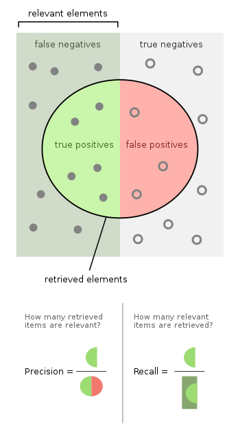
Precision and Recall are performance metrics that allow the evaluation of a classification algorithm. Wikipedia

Precision

What proportion of positive identifications was actually correct? Google Developers

true_positive = confusion_matrix_[1, 1]
false_positive = confusion_matrix_[0, 1]

true_positive / (true_positive + false_positive)

np.float64(0.7931034482758621)

Recall (Sensitivity)

What proportion of actual positives was identified correctly? Google Developers

false_negative = confusion_matrix_[1, 0]

true_positive / (true_positive + false_negative)

np.float64(0.3108108108108108)

Specificity

What proportion of actual negatives was identified correctly? Wikipedia

true_negative = confusion_matrix_[0, 0]

true_negative / (true_negative + false_positive)

np.float64(0.9968847352024922)

Accuracy Score

What is the proportion of correct identifications? Wikipedia

from sklearn.metrics import accuracy_score

accuracy_score(y_test, predictions)

0.9715

or:

true_predictions = confusion_matrix_[0, 0] + confusion_matrix_[1, 1]
true_predictions / len(X_test)

np.float64(0.9715)

statsmodels

Confusion Matrix

prediction_table = sm_estimation.pred_table()
prediction_table

array([[9627.,   40.],
       [ 228.,  105.]])

row_sums = prediction_table.sum(axis=1, keepdims=True)
prediction_table / row_sums

array([[0.99586221, 0.00413779],
       [0.68468468, 0.31531532]])

Regression Report

The regression report is a summary of the regression model. It includes the coefficients, standard errors, t-values, p-values, and confidence intervals for each coefficient.

sm_estimation.summary()

Logit Regression Results

Dep. Variable:	default	No. Observations:	10000
Model:	Logit	Df Residuals:	9996
Method:	MLE	Df Model:	3
Date:	Sun, 11 Jan 2026	Pseudo R-squ.:	0.4619
Time:	15:07:50	Log-Likelihood:	-785.77
converged:	True	LL-Null:	-1460.3
Covariance Type:	nonrobust	LLR p-value:	3.257e-292

	coef	std err	z	P>|z|	[0.025	0.975]
Intercept	-5.9752	0.194	-30.849	0.000	-6.355	-5.596
balance	2.7747	0.112	24.737	0.000	2.555	2.995
income	0.0405	0.109	0.370	0.712	-0.174	0.255
student	-0.6468	0.236	-2.738	0.006	-1.110	-0.184

Possibly complete quasi-separation: A fraction 0.15 of observations can be
perfectly predicted. This might indicate that there is complete
quasi-separation. In this case some parameters will not be identified.