Exercise IX: The Haxby Experiment (2001)#
Thie exercise is based on an example from nilearn’s documentation.
The Haxby Experiment (2001) [1] shows that the representation of objects from different categories is distributed and overlaps over brain regions that were broadly considered to be “specialized” to particular stimuli categories (i.e. the fusiform area for faces and the parahippocampal place area for places).


![]() [Decoding]
[Decoding]


For the purposes of this exercise, we will predict stimulus categories based on the signal acquired from the ventral temporal cortex alone. This demonstration will show that while there was some expected variation, classification performance was relatively high across categories.
Let’s start things off by using nilearn’s datasets module to download a single subjects dataset:
from nilearn import datasets

haxby_data = datasets.fetch_haxby()
[fetch_haxby] Added README.md to /home/runner/nilearn_data
[fetch_haxby] Dataset created in /home/runner/nilearn_data/haxby2001
[fetch_haxby] Downloading data from https://www.nitrc.org/frs/download.php/7868/mask.nii.gz ...
[fetch_haxby]  ...done. (1 seconds, 0 min)

[fetch_haxby] Downloading data from http://data.pymvpa.org/datasets/haxby2001/MD5SUMS ...
[fetch_haxby]  ...done. (1 seconds, 0 min)

[fetch_haxby] Downloading data from http://data.pymvpa.org/datasets/haxby2001/subj2-2010.01.14.tar.gz ...
[fetch_haxby]
Downloaded 110796800 of 291168628 bytes (38.1%%,    1.6s remaining)
[fetch_haxby]
Downloaded 242581504 of 291168628 bytes (83.3%%,    0.4s remaining)
[fetch_haxby] ...done. (3 seconds, 0 min)
[fetch_haxby] Extracting data from /home/runner/nilearn_data/haxby2001/9cabe068089e791ef0c5fe930fc20e30/subj2-2010.01.14.tar.gz...
[fetch_haxby] .. done.
haxby_data
{'anat': ['/home/runner/nilearn_data/haxby2001/subj2/anat.nii.gz'],
 'func': ['/home/runner/nilearn_data/haxby2001/subj2/bold.nii.gz'],
 'session_target': ['/home/runner/nilearn_data/haxby2001/subj2/labels.txt'],
 'mask_vt': ['/home/runner/nilearn_data/haxby2001/subj2/mask4_vt.nii.gz'],
 'mask_face': ['/home/runner/nilearn_data/haxby2001/subj2/mask8b_face_vt.nii.gz'],
 'mask_house': ['/home/runner/nilearn_data/haxby2001/subj2/mask8b_house_vt.nii.gz'],
 'mask_face_little': ['/home/runner/nilearn_data/haxby2001/subj2/mask8_face_vt.nii.gz'],
 'mask_house_little': ['/home/runner/nilearn_data/haxby2001/subj2/mask8_house_vt.nii.gz'],
 'mask': '/home/runner/nilearn_data/haxby2001/mask.nii.gz',
 'description': '.. _haxby_dataset:\n\nHaxby dataset\n=============\n\nAccess\n------\nSee :func:`nilearn.datasets.fetch_haxby`.\n\nNotes\n-----\nResults from a classical :term:`fMRI` study that investigated the differences between\nthe neural correlates of face versus object processing in the ventral visual\nstream. Face and object stimuli showed widely distributed and overlapping\nresponse patterns.\n\nSee :footcite:t:`Haxby2001`.\n\nContent\n-------\nThe "simple" dataset includes:\n    :\'func\': Nifti images with bold data\n    :\'session_target\': Text file containing run data\n    :\'mask\': Nifti images with employed mask\n    :\'session\': Text file with condition labels\n\nThe full dataset additionally includes\n    :\'anat\': Nifti images with anatomical image\n    :\'func\': Nifti images with bold data\n    :\'mask_vt\': Nifti images with mask for ventral visual/temporal cortex\n    :\'mask_face\': Nifti images with face-reponsive brain regions\n    :\'mask_house\': Nifti images with house-reponsive brain regions\n    :\'mask_face_little\': Spatially more constrained version of the above\n    :\'mask_house_little\': Spatially more constrained version of the above\n\nReferences\n----------\n\n.. footbibliography::\n\nFor more information see:\nPyMVPA provides a tutorial using this dataset :\nhttp://www.pymvpa.org/tutorial.html\n\nMore information about its structure :\nhttp://dev.pymvpa.org/datadb/haxby2001.html\n\n\nLicense\n-------\nunknown\n',
 't_r': 2.5}
Review the dataset’s description:
print(haxby_data.description.decode())
---------------------------------------------------------------------------
AttributeError                            Traceback (most recent call last)
Cell In[3], line 1
----> 1 print(haxby_data.description.decode())

AttributeError: 'str' object has no attribute 'decode'
Visualization#
fMRI data is generally represented as a 4D matrix of 3D EPI scans over time.
To read the fMRI volume from a .nii.gz file we’ll use nibabel’s load() function:
from nilearn import plotting
import nibabel as nib

fmri_path = haxby_data.func[0]
fmri_data = nib.load(fmri_path)
fmri_data.shape
(40, 64, 64, 1452)
To plot a 3D image representing the mean fMRI signal over time for the single subject in the dataset:
from nilearn.image import mean_img

fmri_mean_epi = mean_img(fmri_data)
plotting.view_img(fmri_mean_epi, threshold=None)
Masking#
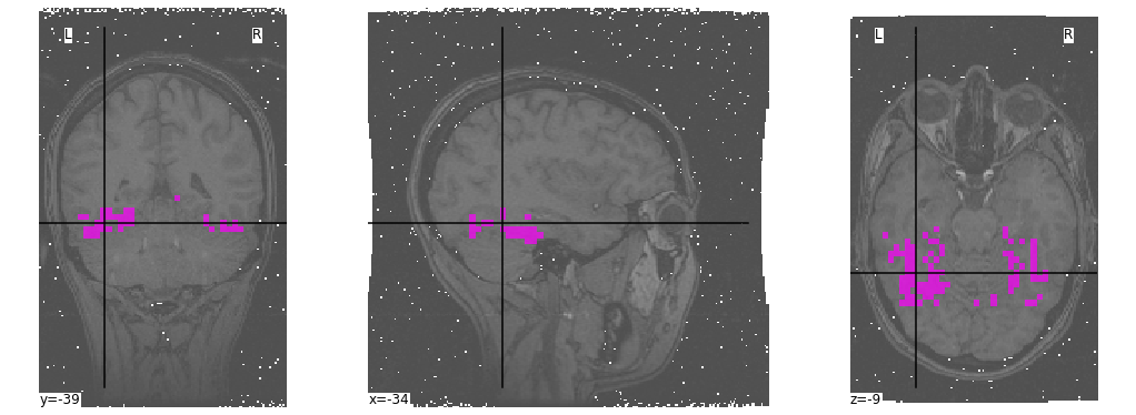
In order to analyze the data, we need to produce a matrix containing the measured signal in the ventral temporal (VT) cortex over time.
First, let’s have a look at the provided mask:
import matplotlib.pyplot as plt

mask = haxby_data.mask_vt[0]
anatomical = haxby_data.anat[0]

figure = plt.figure(figsize=(14, 5))
_ = plotting.plot_roi(mask,
                      bg_img=anatomical,
                      cmap="spring",
                      black_bg=False,
                      figure=figure)
Now, we will use this ROI in order to mask our 4D fMRI data:

from nilearn.input_data import NiftiMasker

masker = NiftiMasker(mask_img=mask, standardize=True)
masked_data = masker.fit_transform(fmri_data)
The result containts time points as rows and voxels as columns:
masked_data.shape
(1452, 464)
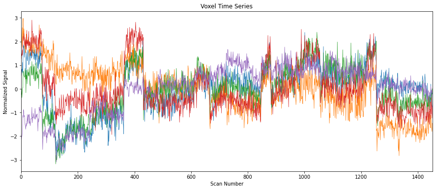
For example, to plot the change in the measured signal in some 5 voxels over time:
START_VOXEL, END_VOXEL = 0, 5
SIGNAL_PLOT_CONFIGURATION = {
    "title": "Voxel Time Series",
    "xlabel": "Scan Number",
    "ylabel": "Normalized Signal",
    "xlim": (0, len(masked_data))
}

fig, ax = plt.subplots(figsize=(15, 6))
ax.plot(masked_data[:, START_VOXEL:END_VOXEL], linewidth=0.75)
_ = ax.set(**SIGNAL_PLOT_CONFIGURATION)
Prediction#
Let’s try and predict which stimulus category the subject was viewing based on the masked fMRI data.
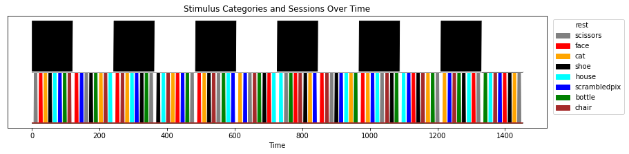
Reading the labels#
The session_target file contains a labels column, describing the stimulus category at each presentation block, as well as the session (chunks) out of 12 sessions presented to each subjects.
import pandas as pd

LABEL_COLUMNS = {'labels': 'Label', 'chunks': 'Session'}

labels_path = haxby_data.session_target[0]
labels = pd.read_csv(labels_path, delimiter=' ')
labels.rename(columns=LABEL_COLUMNS, inplace=True)
labels
| Label | Session | |
|---|---|---|
| 0 | rest | 0 |
| 1 | rest | 0 |
| 2 | rest | 0 |
| 3 | rest | 0 |
| 4 | rest | 0 |
| ... | ... | ... |
| 1447 | rest | 11 |
| 1448 | rest | 11 |
| 1449 | rest | 11 |
| 1450 | rest | 11 |
| 1451 | rest | 11 |
1452 rows × 2 columns
Let’s create a couple of references to the given data for comfort and readability.
is_task = labels["Label"] != 'rest'

task_data = masked_data[is_task]
task_labels = labels["Label"][is_task]
task_sessions = labels["Session"][is_task]

categories = task_labels.unique()
Logistic Regression#
To grid search across \(\ell_1\) and \(\ell_2\) with various C values and score based on the ROC AUC:
from sklearn.linear_model import LogisticRegression
from sklearn.model_selection import GridSearchCV, LeaveOneGroupOut

SOLVER = "liblinear"  # See note 1
model = LogisticRegression(random_state=0, solver=SOLVER)
C = [10**i for i in range(-2, 3)]
PARAM_GRID = {"C": C, "penalty": ["l1", "l2"]}
SCORING = "roc_auc"

searcher = GridSearchCV(model,
                        param_grid=PARAM_GRID,
                        scoring=SCORING,
                        cv=LeaveOneGroupOut())  # See note 2
Note
sklearn offers a variety of different solvers for logistic regression, in our case we need to make sure we use one that supports both \(\ell_1\) and \(\ell_2\) regularization. For more information, see the LogistricRegression model’s user guide.
Note
The fMRI data is acquired by sessions, and the noise is autocorrelated in a given session. Hence, it is better to predict across sessions when doing cross-validation.
Our goal now it to evaluate how well we manage to classify the target category of stimuli based on the signal from the verntral temporal cortex alone:
# Create a DataFrame to store the results
scores = pd.DataFrame(index=categories, columns=["Penalty", "C", "AUC"])

# Iterate categories and updates best scores
for category in categories:
    target = task_labels == category
    searcher.fit(
        X=task_data,
        y=target,
        groups=task_sessions,
    )
    cv_results = searcher.cv_results_
    scores.loc[category, "Penalty"] = searcher.best_estimator_.penalty
    scores.loc[category, "C"] = searcher.best_estimator_.C
    scores.loc[category, "AUC"] = searcher.best_score_
scores
| Penalty | C | AUC | |
|---|---|---|---|
| scissors | l2 | 10 | 0.912551 |
| face | l1 | 1 | 0.986919 |
| cat | l2 | 100 | 0.961052 |
| shoe | l2 | 1 | 0.925779 |
| house | l1 | 0.1 | 0.998089 |
| scrambledpix | l1 | 10 | 0.989418 |
| bottle | l1 | 1 | 0.898883 |
| chair | l1 | 10 | 0.93107 |
Not bad! Clearly, the ventral temporal cortex has some significant value in decoding the represenation of the various stimulus categories (and not just faces).